7|PROBABILITY

Overview

Probability basics
Sampling
Probability and distributions
Probability and \(z\)-scores
Learning checks

Probability basics

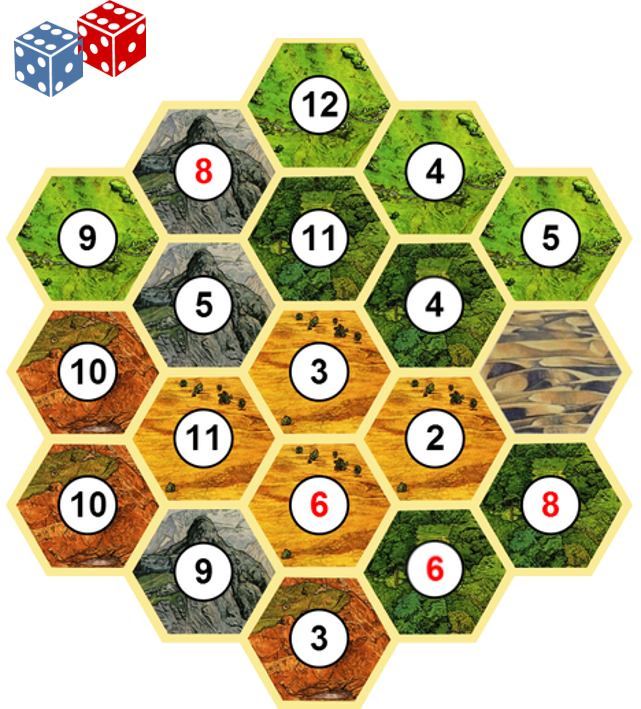
Probability and games

Settlers of Catan
- Board of hex tiles, each with a number
- Place “settlements” at intersection of tiles
- Each turn, roll 2 dice
- You get resources if your settlement is touching the rolled total
- Where do you put your first settlement?

Definition & notation

Several different outcomes are possible
- The probability of any specific outcome is a fraction of all possible outcomes
- \(p\) is the symbol for “probability”
- Probability of some specific outcome is specified by \(p(event)\)

\(p(A) = \dfrac{number \ of \ outcomes \ classified \ as \ A}{total \ number \ of \ possible \ outcomes}\)

Example: coin flip

E.g. Flipping a coin
- Numerator: number of those outcomes
- Denominator: all possible outcomes

\(p(heads) = 1/2 = .5\)

\(p(tails) = 1/2 = .5%\)

Example: rolling dice

All possible outcomes:
1, 2, 3, 4, 5, 6

\(p(6) = 1/6 = 0.17\)

\(p(1) = 1/6 = 0.17\)

\(p(odd) = 3/6 = 0.5\)

Example: rolling 2 dice

\(p(2) = 1/36 = .03\)
\(p(12) = 1/36 = .03\)
\(p(7) = 6/36 = .17\)

Roll	1	2	3	4	5	6
1	2	3	4	5	6	7
2	3	4	5	6	7	8
3	4	5	6	7	8	9
4	5	6	7	8	9	10
5	6	7	8	9	10	11
6	7	8	9	10	11	12

Sampling

Sampling marbles

Jar of marbles
- Contains 25 white & 25 blue marbles
- What is the probability of randomly drawing a white marble?
- Number of those outcomes (25)
- Divided by total number of outcomes (50)

\(p(white) = 25/50 = .5\)

More marbles

Different jar
- 40 blue & 10 white marbles
- What is the probability of randomly drawing a white marble?

\(p(white) = 10/50 = .2\)

Repeated sampling

Repeated sampling
- 40 blue, 10 white
- What is the probability of randomly drawing one white marble and then drawing a second white marble?

\(p(first \ white) = 10/50 = .2\)

\(p(second \ white)\) depends on whether we put the first one back or not

Repeated sampling

Without replacement

\[\begin{align} p(white) & = 10/50 = .2 \\ p(second \ white) & = 9/49 \approx .18 \\ p(both \ white) & = .2 * .18 \approx .037 \end{align}\]

With replacement

\(\begin{align} p(white) &= 10/50 = .2 \\ p(second \ white) &= 10/50 = .2 \\ p(both \ white) &= .2 * .2 = .04\end{align}\)

Random sampling

“Random sample” definition
- A sample produced by a process that assures:
  1. Each individual in the population has an equal chance of being selected
  2. Probability of being selected stays constant from one selection to the next when more than one individual is selected
- “Independent random sampling”
Requires sampling with replacement

Probability and distributions

\(p(X = 1) = 4/10 = 0.4\)

\(p(X \ge 4) = 3/10 = 0.3\)

\(p(1 \lt X \lt 5) = 5/10 = .5\)

Probability and z-scores

Normal distribution
- Symmetrical
- Highest frequency in the middle
- Tapers off towards the extremes
- Very common distribution shape
- Defined by an equation
- Can be described by the proportions of area contained in each section

\(Y = \dfrac{1}{\sqrt{2 \pi \sigma^2}}e^{-(X-\mu)^2 / 2\sigma^2}\)

Unit Normal Table

\(z\)	Proportion in body	Proportion in tail	Proportion between \(M\) and \(z\)
0.0	0.5000	0.5000	0.0000
0.1	0.5398	0.4602	0.0398
0.2	0.5793	0.4207	0.0793
0.3	0.6179	0.3821	0.1179
0.4	0.6554	0.3446	0.1554
0.5	0.6915	0.3085	0.1915
0.6	0.7257	0.2743	0.2257
0.7	0.7580	0.2420	0.2580
0.8	0.7881	0.2119	0.2881
0.9	0.8159	0.1841	0.3159
1.0	0.8413	0.1587	0.3413
1.1	0.8643	0.1357	0.3643
1.2	0.8849	0.1151	0.3849
1.3	0.9032	0.0968	0.4032
1.4	0.9192	0.0808	0.4192
1.5	0.9332	0.0668	0.4332
1.6	0.9452	0.0548	0.4452
1.7	0.9554	0.0446	0.4554
1.8	0.9641	0.0359	0.4641
1.9	0.9713	0.0287	0.4713
2.0	0.9772	0.0228	0.4772

Unit Normal Table

\(z\)	Proportion in body	Proportion in tail	Proportion between \(M\) and \(z\)
0.0	0.5000	0.5000	0.0000
0.1	0.5398	0.4602	0.0398
0.2	0.5793	0.4207	0.0793
0.3	0.6179	0.3821	0.1179
0.4	0.6554	0.3446	0.1554
0.5	0.6915	0.3085	0.1915
0.6	0.7257	0.2743	0.2257
0.7	0.7580	0.2420	0.2580
0.8	0.7881	0.2119	0.2881
0.9	0.8159	0.1841	0.3159
1.0	0.8413	0.1587	0.3413
1.1	0.8643	0.1357	0.3643
1.2	0.8849	0.1151	0.3849
1.3	0.9032	0.0968	0.4032
1.4	0.9192	0.0808	0.4192
1.5	0.9332	0.0668	0.4332
1.6	0.9452	0.0548	0.4452
1.7	0.9554	0.0446	0.4554
1.8	0.9641	0.0359	0.4641
1.9	0.9713	0.0287	0.4713
2.0	0.9772	0.0228	0.4772

Using R

pnorm(0.2)  # area to the left of z = 0.2

[1] 0.5792597

pnorm(0.2, lower.tail=FALSE) # area to the right of z = 0.2

[1] 0.4207403

# can specify different mean & SD
pnorm(700, mean=500, sd=100, lower.tail=FALSE)

[1] 0.02275013

# can specify proportion & find corresponding score
qnorm(.0228, mean=500, sd=100, lower.tail=FALSE)

[1] 699.9077

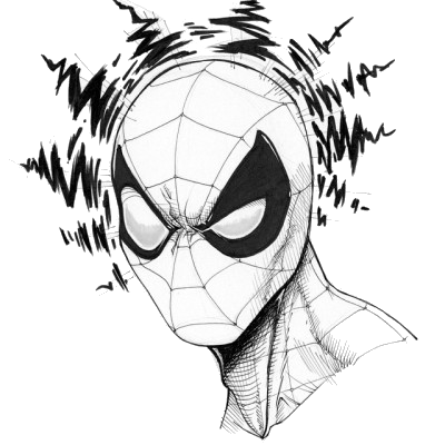
Spiderman

Are Peter Parker’s RTs “noticeably different?”
- \(z = -2.5\)
- Can state precise probability of observing a \(z\)-score that (or more) extreme

pnorm(-2.5)

[1] 0.006209665

pnorm(159, mean = 284, sd = 50)

[1] 0.006209665

Warning

Probabilities given in the Unit Normal Table will be accurate only for normally distributed scores
- Shape of the distribution must be verified
- Important assumption of Central Limit Theorem

Learning checks

Which (if any) of the following meet the definition of a true random sample?

Several contestants spinning the wheel on The Price is Right to pick a number
Standing on the street and surveying people who happen to walk by
Getting Intro Psych students to participate in return for course credit
Calling random phone numbers from a database

table_selection = {
  var num = 0
  
  function getNumberFromTable() {
    try {
      num = d3.select(this).select("td")._groups[0][0].innerHTML;
    } catch {} finally {update();}
  }
  
  d3.select("#tbl").selectAll("tr").on("mouseover", getNumberFromTable)
  
  const w = 500
  const h = 400
  
  const margins = {t: 50, r: 10, b: 50, l: 10}
  
  const x = d3.scaleLinear()
    .domain([-3,3])
    .range([margins.l,w-margins.r])
  const y = d3.scaleLinear()
    .domain([0,0.41])
    .range([h-margins.b,margins.t])
  const line = d3.line()
    .x(d => x(d.value))
    .y(d => y(d.density))
  const axis = d3.axisBottom(x)
  
  const svg = d3.select("#z-container")
    .append("svg").attr("width", w).attr("height", h)
  
  svg.append("g")
    .call(axis)
    .attr("transform", "translate(0," + y(0) +")")
  
  svg.append("path").attr("d", line(curve))
    .style("stroke", "black").style("fill", "none")
    .attr("class", "invertable")
    
  svg.append("path")
    .style("fill", "thistle").style("fill-opacity", 0.5)
    .attr("d", line(curve))
    
  svg.append("path")
    .style("fill", "thistle").style("fill-opacity", 0.5)
    .attr("d", line(curve))
    .attr("clip-path", "url(#clip)")

    
  function update() {
  
  svg.selectAll("clipPath").remove()
  svg.append("clipPath").attr("id", "clip")
    .append("rect")
    .attr("width", x(num))
    .attr("height", h)
  }
  
  update();
}