8|SAMPLING

Overview

Sampling error
Distribution of sample means
Central Limit Theorem
Learning checks

Roadmap

So far…
- \(z\)-scores describe the location of a single score in a sample or in a population
- Normal distributions: precisely quantify probability of obtaining certain scores
Moving forward…
- Quantifying probability of obtaining certain sample statistics

Sampling error

Error: Discrepancy between a sample statistic and the population parameter

import { pop } from "./02_variables.qmd";

Sampling error

Discrepancy between a sample statistic and the population parameter
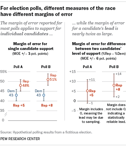
- E.g. Opinion polling
- see Pew explainer

Sampling error: IQ

Distribution of Sample Means

“Distribution of Sample Means” / “Sampling distribution of the mean”
- Distribution of sample means obtained by selecting all possible samples of size \(n\) from a population
- Often huge number of possible samples
- But distribution forms a simple & predictable pattern

Characteristics

Shape
- The distribution will be approximately normal
- Sample \(M\)s are representative of population \(\mu\)
- Most means will be close to \(\mu\); means far from \(\mu\) are rare
Center
- The center/average of the distribution will be close to \(\mu\)
- \(M\) is a unbiased statistic
- On average, \(M = \mu\)
Variability
- Related to sample size, \(n\)
- The larger the sample, the less the variability
- Larger samples are more representative

Example: height distribution

Sample	X1	X2	M
1	60	60	60
2	62	60	61
3	64	60	62
4	66	60	63
5	60	62	61
6	62	62	62
7	64	62	63
8	66	62	64
9	60	64	62
10	62	64	63
11	64	64	64
12	66	64	65
13	60	66	63
14	62	66	64
15	64	66	65
16	66	66	66

Sampling distribution (\(n = 2\))

\(p(M < 61) =\ ?\)

\(p(62 \le M \le 64) =\ ?\)

\(p(M > 65) =\ ?\)

Example: height distribution

Now we can calculate variability of sample means
- Since we obtained every sample mean
- Use population SD formula

\(X\)	\(X-M\)	\((X-M)^2\)
60	-3	9
61	-2	4
62	-1	1
63	0	0
61	-2	4
62	-1	1
63	0	0
64	1	1
62	-1	1
63	0	0
64	1	1
65	2	4
63	0	0
64	1	1
65	2	4
66	3	9
\(M = 63.00\)		\(SS = 40.00\)
		\(\sigma^2 = 2.50\)
		\(\sigma = 1.58\)

Central Limit Theorem

Sampling & the Central Limit Theorem
- Distribution of samples means based on all possible samples from a population not feasible in most realistic situations
- But we can mathematically predict shape, mean, & variability for any sample size & population

Central Limit Theorem

For any population with mean \(\mu\) and standard deviation \(\sigma\), the distribution of sample means for sample size \(n\) will have…
- An expected mean \(\mu_M\) of \(\mu\)
- A standard deviation of \(\dfrac{\sigma} {\sqrt{n}}\)
- And will approach a normal distribution as \(n\) approaches infinity

Shape

Almost perfectly normal in either of two conditions
- The population from which the samples are selected is a normal distribution
- Or…
- Sample \(n\)s are relatively large

…what is relatively large?
- As \(n\) approaches infinity, distribution of sample means approaches a normal distribution
- But by \(n = 30\) means pile up symmetrically around \(\mu\)
- Population distribution does not need to be normal; can be skewed, flat, bimodal, whatever

Mean

Mean of the distribution of sample means is called the expected value of \(M\) ( \(\mu_M\) )
- On average, \(M = \mu_M = \mu\)
- \(M\) is unbiased
- If we only have a single sample \(M\), our best guess at the (unknown) population mean should always be the (known) sample mean
- But we can acknowledge variability…

Variability

Standard deviation of the sample means
- “Standard error of the mean”; \(\sigma_M\)
- Measure of how well a sample mean estimates its population mean
- How much sampling error we can expect; how much distance is expected on average between \(M\) and \(\mu\)

\(\sigma_M = \dfrac{\sigma}{\sqrt{n}}\) or \(\dfrac{\sqrt{\sigma^2}}{\sqrt{n}}\) or \(\sqrt{\dfrac{\sigma^2}{n}}\)

Variability

μ =

σ =

n = 30

σ_M =

Variability: heights sampling dist

Sample	X1	X2	M
1	60	60	60
2	62	60	61
3	64	60	62
4	66	60	63
5	60	62	61
6	62	62	62
7	64	62	63
8	66	62	64
9	60	64	62
10	62	64	63
11	64	64	64
12	66	64	65
13	60	66	63
14	62	66	64
15	64	66	65
16	66	66	66

Sampling distribution (\(n = 2\))

\(\sigma_M = \dfrac{\sigma}{\sqrt{n}} = \dfrac{2.24}{\sqrt{2}} = 1.58\)

Summary

Summary
- Distribution of sample means for samples of size \(n\) will have…
  - a mean of \(\mu_M\)
  - standard deviation \(\sigma_M = \sigma / \sqrt{n}\)
  - Shape will be normal if population is normally distributed, or \(n > 30\)

Learning checks

True or False?
- The mean of a sample is always equal to the population mean
- The shape of a distribution of sample means is always normal
- As sample size increases, the value of the standard error always decreases
Describe the distribution of sample means (shape, expected value of the mean, and standard error) for samples of \(n = 100\) selected from a population with \(\mu = 40\) and \(\sigma = 10\).

Galton board

import { board } from "../ojs/galton-board.qmd"

cover = {
  const w = 1050
  const h = 500
  
  const xScale = d3.scaleLinear()
    .domain([25, 175])
    .range([0, w])
  const yScale = d3.scaleLinear()
    .domain([0, 70])
    .range([h, 0])
  
  const svg = d3.select("#cover-container")
    .append("svg")
    .attr("width", w).attr("height", h)

svg.selectAll("rect")
  .data(data)
  .enter()
  .append("rect")
    .attr("class", "invertable")
    .attr("x", d => xScale(d.xValue))
    .attr("y", d => yScale(d.y_cum))
    .attr("width", 5)
    .attr("height",5)
    .style("fill", "black")
    .style("stroke", "none")
    .style("opacity", 0)
    .transition().duration(0).delay((d,i) => i*2)
      .style("opacity", 1)

}

sampling_chart = {

  const w = 1050
  const h = 500
  const margin = ({top: 20, right: 200, bottom: 100, left: 200})
  const xlims = [75, 125]
  const xRange = xlims[1] - xlims[0]
  const x = d3.scaleLinear()
    .domain(xlims)
    .range([margin.left, w - margin.right])

  const max_y = Math.max(...samples.map(o => o.count))

  const y = d3.scaleLinear()
    .domain([0, max_y])
    .range([h - margin.bottom, margin.top])

  const xAxis = d3.axisBottom(x).ticks(8)

  d3.select("#sampling-chart").select("svg").remove()
  
  const svg =  d3.select("#sampling-chart")
    .append("svg").attr("width", w).attr("height", h)
    
  const controls = svg.append("g").attr("transform", `translate(0,${h-margin.bottom/2})`)
  
  var quantity = 500;

  const buttonData = [{id: "reset", text: "↻"},
                      {id: "next", text: "ᐳ"},
                      {id: "play", text: "►"}]
                      
  
  const buttons = controls.append("g")
    .attr("transform", `translate(0, 20)`)
    
  buttons.selectAll("text")
    .data(buttonData)
    .enter().append("text")
    .attr("id", d => "button-" + d.id)
    .attr("class", "button")
    .text(d => d.text)
    .attr("x", (d,i) => 400 + i * 75)
  
  var playing = false;
  d3.select("#button-reset").on("click", reset)
  d3.select("#button-next").on("click", drawOne)
  d3.select("#button-play").on("click", playClicked)
  
  const g = svg.append("g").attr("id", "boxes")
  
  function playButtonText() {
    d3.select("#button-play").text(function(){
      if(playing & quantity < samples.length) {
        return "◼"
      } else {
        return "▶"
      }
    })
  }
  
  function reset() {
    playing = false;
    playButtonText();
    quantity = 0;
    drawBoxes();
    d3.select("#sampling-info")
      .html("Observations: " + '<br/>' + "<i>M</i> = ")
  }
  
  function drawOne() {
  if (quantity >= samples.length) {
    playing = false;
    return false
  }
    quantity++;
    drawBoxes();
    describeSample();
  }
  

  
  function playClicked() {
    playing = !playing
    
    playButtonText();
  
    if(playing) {
      drawContinuously();
    }
  }
  
  const sleep = (milliseconds) => {
    return new Promise(resolve => setTimeout(resolve, milliseconds))
  }
  
  function drawContinuously() {
    if(playing) {
      drawOne();
      sleep(10).then(drawContinuously);
    }
  }
  
  function drawBoxes() {
  g.selectAll("rect").remove()
  g.selectAll("rect")
    .data(samples.slice(0, quantity))
    .enter()
    .append("rect")
      .attr("class", "invertable")
      .attr("fill", "black")
      .attr("stroke", "none")
      .attr("x", d => x(d.mean_bin - 0.5))
      .attr("y", d => y(d.count))
      .attr("width", (w-margin.left-margin.right)/xRange * 0.9)
      .attr("height", (h-margin.top-margin.bottom)/max_y * 0.9)
      .each(function (d, i) {
            if (i === quantity-1) {
              // put all your operations on the second element, e.g.
              d3.select(this).attr("fill", "red");    
            }
          })
  }
  svg.append("g").attr("id", "xaxis")
      .call(xAxis)
      .attr("transform", `translate(0,${y(0)})`)
      .attr("class", "axis")
      .style("font-size", "0.5em");
  
  d3.select("#sampling-info")
      .style("font-family", "KaTeX_Main")
      .style("font-size", "0.9em")
      .html("Observations:<br/><span style='font-style: italic;'>M =</span>")
      
  function describeSample() {
    d3.select("#sampling-info")
      .style("font-family", "KaTeX_Main")
      .style("font-size", "0.9em")
      .html("Observations: " + samples[quantity-1].sample.join(", ") + '<br/>' + "<i>M</i> = " + samples[quantity-1].mean)
  }
  
  drawBoxes();
  describeSample();
}

jStat = require("https://cdn.jsdelivr.net/npm/jstat@latest/dist/jstat.min.js")


chart = {

  const w = 1050
  const h = 600
  var mu = 100
  var sigma = 15
  var n = 30
  var std_err = sigma/Math.sqrt(n)
  var max_std_err = sigma / Math.sqrt(50)
  
  const margin = ({top: 20, right: 0, bottom: 30, left: 0})

  var xlim = [mu - 3 * sigma, mu + 3 * sigma]

  var x = d3.scaleLinear()
    .domain([xlim[0], xlim[1]])
    .range([margin.left, w - margin.right])
  const y = d3.scaleLinear()
    .domain([0, jStat.normal.pdf(mu, mu, max_std_err)])
    .range([h - margin.bottom, margin.top])
  const line = d3.line()
    .x(d => x(d.value))
    .y(d => y(d.density))
  
  var xAxis = d3.axisBottom(x).ticks(10);
  
  function makeCurve(mu, sm) {
    var values = jStat(xlim[0], xlim[1], 210)[0],
        arr = [];
    for (var i in values) {
      arr.push({
          value: values[i], 
          density: jStat.normal.pdf(values[i], mu, sm)
      })
    }
    return arr;
  }
  

  
  const svg = d3.select("#sampling-distribution-container").append("svg")
    .attr("width", w)
    .attr("height", h)

  var axis = svg.append("g")
      .attr("transform", `translate(0,${y(0)})`)
  
  const popCurve = svg.append("path")
      .attr("fill", "none")
      .attr("stroke", "black")
      .attr("opacity", 0.5)
      .attr("stroke-width", 1.5)
      .attr("stroke-dasharray", [10, 10])
      .attr("class", "invertable");
      
  const curve = svg.append("path")
      .style("fill", "var(--link-color)")
      .style("fill-opacity", 0.5)
      .style("stroke", "var(--text-color)")
      .style("stroke-width", 4);
      
  const f = d3.format(".2f")
  
  
 
  const changeMu = function(e) {
    mu = Number(e.target.value);
    updateAxis();
    redrawCurves();
  }
  
  const muInput = document.getElementById('mu-input')
 muInput.addEventListener('input', changeMu);
 
  const changeSigma = function(e) {
    sigma = Number(e.target.value);
    std_err = sigma/Math.sqrt(n);
    updateValues();
    updateAxis();
    redrawCurves();
  }
  
  const sigmaInput = document.getElementById('sigma-input')
 sigmaInput.addEventListener('input', changeSigma);


  
  const nInput = document.getElementById('n-input')
  nInput.oninput = function() {
    n = nInput.value
    std_err = sigma/Math.sqrt(n)
    updateValues();
    redrawSamplingDistCurve();
  };
  
  
  function updateValues() {
    d3.select("#n-value").text(n)
    d3.select("#std-err-value")
      .text(f(std_err))
  }
  
  function redrawSamplingDistCurve() {
    curve.attr("d", line(makeCurve(mu, std_err)))
  };
  
  function redrawPopulationCurve() {
    popCurve.attr("d", line(makeCurve(mu, sigma)))
  };
  
  function redrawCurves() {
    redrawSamplingDistCurve();
    redrawPopulationCurve();
  }
  
  function updateAxis() {
    max_std_err = sigma / Math.sqrt(50)
    y.domain([0, jStat.normal.pdf(mu, mu, max_std_err)])
    
    xlim = [mu - 3 * sigma, mu + 3 * sigma];
    console.log(xlim);
    x.domain([xlim[0], xlim[1]]);
    xAxis = d3.axisBottom(x).ticks(10);
    
    axis.select("g").remove();
    axis.append("g").call(xAxis).style("font-size", "0.6em")
  }

  updateAxis();
  updateValues();
  redrawCurves();
  
  
}

Sample	X1	X2	M
1	60	60	60
2	62	60	61
3	64	60	62
4	66	60	63
5	60	62	61
6	62	62	62
7	64	62	63
8	66	62	64
9	60	64	62
10	62	64	63
11	64	64	64
12	66	64	65
13	60	66	63
14	62	66	64
15	64	66	65
16	66	66	66

Sample	X1	X2	M
1	60	60	60
2	62	60	61
3	64	60	62
4	66	60	63
5	60	62	61
6	62	62	62
7	64	62	63
8	66	62	64
9	60	64	62
10	62	64	63
11	64	64	64
12	66	64	65
13	60	66	63
14	62	66	64
15	64	66	65
16	66	66	66

Sample	X1	X2	M
1	60	60	60
2	62	60	61
3	64	60	62
4	66	60	63
5	60	62	61
6	62	62	62
7	64	62	63
8	66	62	64
9	60	64	62
10	62	64	63
11	64	64	64
12	66	64	65
13	60	66	63
14	62	66	64
15	64	66	65
16	66	66	66

Sample	X1	X2	M
1	60	60	60
2	62	60	61
3	64	60	62
4	66	60	63
5	60	62	61
6	62	62	62
7	64	62	63
8	66	62	64
9	60	64	62
10	62	64	63
11	64	64	64
12	66	64	65
13	60	66	63
14	62	66	64
15	64	66	65
16	66	66	66

Sample	X1	X2	M
1	60	60	60
2	62	60	61
3	64	60	62
4	66	60	63
5	60	62	61
6	62	62	62
7	64	62	63
8	66	62	64
9	60	64	62
10	62	64	63
11	64	64	64
12	66	64	65
13	60	66	63
14	62	66	64
15	64	66	65
16	66	66	66

Sample	X1	X2	M
1	60	60	60
2	62	60	61
3	64	60	62
4	66	60	63
5	60	62	61
6	62	62	62
7	64	62	63
8	66	62	64
9	60	64	62
10	62	64	63
11	64	64	64
12	66	64	65
13	60	66	63
14	62	66	64
15	64	66	65
16	66	66	66